Requirement already satisfied: kaggle in /usr/local/lib/python3.6/dist-packages (1.5.9)
Requirement already satisfied: requests in /usr/local/lib/python3.6/dist-packages (from kaggle) (2.23.0)
Requirement already satisfied: tqdm in /usr/local/lib/python3.6/dist-packages (from kaggle) (4.41.1)
Requirement already satisfied: python-slugify in /usr/local/lib/python3.6/dist-packages (from kaggle) (4.0.1)
Requirement already satisfied: urllib3 in /usr/local/lib/python3.6/dist-packages (from kaggle) (1.24.3)
Requirement already satisfied: certifi in /usr/local/lib/python3.6/dist-packages (from kaggle) (2020.6.20)
Requirement already satisfied: six>=1.10 in /usr/local/lib/python3.6/dist-packages (from kaggle) (1.15.0)
Requirement already satisfied: python-dateutil in /usr/local/lib/python3.6/dist-packages (from kaggle) (2.8.1)
Requirement already satisfied: slugify in /usr/local/lib/python3.6/dist-packages (from kaggle) (0.0.1)
Requirement already satisfied: chardet<4,>=3.0.2 in /usr/local/lib/python3.6/dist-packages (from requests->kaggle) (3.0.4)
Requirement already satisfied: idna<3,>=2.5 in /usr/local/lib/python3.6/dist-packages (from requests->kaggle) (2.10)
Requirement already satisfied: text-unidecode>=1.3 in /usr/local/lib/python3.6/dist-packages (from python-slugify->kaggle) (1.3)
3. Kaggle Token 다운로드
Kaggle에서 API Token을 다운로드한다. [Kaggle] - [My Account] - [API] - [Create New API Token]을 누르면 kaggle.json 파일이 다운로드 된다. 파일을 바탕화면에 옮긴 뒤, 아래 코드를 실행한다.
1 2 3 4 5 6 7 8
from google.colab import files uploaded = files.upload() for fn in uploaded.keys(): print('uploaded file "{name}" with length {length} bytes'.format( name=fn, length=len(uploaded[fn]))) # kaggle.json을 아래 폴더로 옮긴 뒤, file을 사용할 수 있도록 권한을 부여한다. !mkdir -p ~/.kaggle/ && mv kaggle.json ~/.kaggle/ && chmod 600 ~/.kaggle/kaggle.json
Saving kaggle.json to kaggle.json
uploaded file "kaggle.json" with length 62 bytes
아래 코드를 실행했을 때, 에러 메시지가 없으면 json 파일이 성공적으로 업로드 되었다는 뜻이다.
# 실습: 타이타닉 데이터 불러오기 !kaggle competitions download -c titanic
Warning: Looks like you're using an outdated API Version, please consider updating (server 1.5.9 / client 1.5.4)
Downloading train.csv to /content/drive/My Drive/Colab Notebooks/Python/python/practice/data
0% 0.00/59.8k [00:00<?, ?B/s]
100% 59.8k/59.8k [00:00<00:00, 8.18MB/s]
Downloading gender_submission.csv to /content/drive/My Drive/Colab Notebooks/Python/python/practice/data
0% 0.00/3.18k [00:00<?, ?B/s]
100% 3.18k/3.18k [00:00<00:00, 443kB/s]
Downloading test.csv to /content/drive/My Drive/Colab Notebooks/Python/python/practice/data
0% 0.00/28.0k [00:00<?, ?B/s]
100% 28.0k/28.0k [00:00<00:00, 3.97MB/s]
1
!ls # ls: 리눅스 명령어, 경로 내 모든 데이터 파일을 보여줌
gender_submission.csv test.csv train.csv
총 3개의 데이터가 다운로드 되었다.
gender_submission.csv
test.csv
train.csv
II. Kaggle Data 실습_Titanic
데이터 살펴보기
Kaggle Code 필사
1. 데이터 살펴보기
아래 코드를 실행하여 EDA 필수 패키지를 설치한다.
1
2
3
4
5
6
7
8
9
10
import pandas as pd # 데이터 가공, 변환 import pandas_profiling # 보고서 기능 import numpy as np # 수치 연산&배열, 행렬 import matplotlib as mpl # 시각화 import matplotlib.pyplot as plt # 시각화 from matplotlib.pyplot import figure # 시각화 import seaborn as sns
from IPython.core.display import display, HTML from pandas_profiling import ProfileReport
gender = pd.read_csv('data/gender_submission.csv') train = pd.read_csv('data/train.csv') test = pd.read_csv('data/test.csv') print("data import is done")
data import is done
(2) 데이터 확인 Kaggle 데이터를 불러와서 가장 먼저 확인해야 할 것은 데이터셋의 크기다.
변수의 개수
Numeric 변수 & Categorical 변수의 개수 등 파악 cf) 보통 test 데이터의 변수 개수가 train 변수 개수보다 하나 적음
1
gender.shape, train.shape, test.shape
((418, 2), (891, 12), (418, 11))
1 2
# train 데이터의 상위 5개 데이터만 확인해보기 display(train.head())
PassengerId
Survived
Pclass
Name
Sex
Age
SibSp
Parch
Ticket
Fare
Cabin
Embarked
0
1
0
3
Braund, Mr. Owen Harris
male
22.0
1
0
A/5 21171
7.2500
NaN
S
1
2
1
1
Cumings, Mrs. John Bradley (Florence Briggs Th...
female
38.0
1
0
PC 17599
71.2833
C85
C
2
3
1
3
Heikkinen, Miss. Laina
female
26.0
0
0
STON/O2. 3101282
7.9250
NaN
S
3
4
1
1
Futrelle, Mrs. Jacques Heath (Lily May Peel)
female
35.0
1
0
113803
53.1000
C123
S
4
5
0
3
Allen, Mr. William Henry
male
35.0
0
0
373450
8.0500
NaN
S
Numerical 변수와 Categorical 변수를 구분한다.
numeric_features 구분
1 2 3 4 5 6 7
numeric_features = train.select_dtypes(include=[np.number]) print(numeric_features.columns) print("The total number of numeric features are: ", len(numeric_features.columns))
numeric_features = test.select_dtypes(include=[np.number]) print(numeric_features.columns) print("The total number of numeric features are: ", len(numeric_features.columns))
Index(['PassengerId', 'Survived', 'Pclass', 'Age', 'SibSp', 'Parch', 'Fare'], dtype='object')
The total number of numeric features are: 7
Index(['PassengerId', 'Pclass', 'Age', 'SibSp', 'Parch', 'Fare'], dtype='object')
The total number of numeric features are: 6
train의 numeric 데이터는 7개, test의 numeric 데이터는 6개이다.
numeric_features 제외한 나머지 변수 추출
1 2 3 4 5 6 7
categorical_features = train.select_dtypes(exclude=[np.number]) print(categorical_features.columns) print("The total number of non numeric features are: ", len(categorical_features.columns))
categorical_features = test.select_dtypes(exclude=[np.number]) print(categorical_features.columns) print("The total number of non numeric features are: ", len(categorical_features.columns))
Index(['Name', 'Sex', 'Ticket', 'Cabin', 'Embarked'], dtype='object')
The total number of non numeric features are: 5
Index(['Name', 'Sex', 'Ticket', 'Cabin', 'Embarked'], dtype='object')
The total number of non numeric features are: 5
train의 numeric 아닌 데이터는 5개, test의 numeric 아닌 데이터는 5개이다.
Finding any relations or trends considering multiple features
1 2 3 4 5 6 7 8 9
# 사용 함수 import import numpy as np import pandas as pd import matplotlib.pyplot as plt import seaborn as sns plt.style.use('fivethirtyeight') import warnings warnings.filterwarnings('ignore') %matplotlib inline
1
train.head()
PassengerId
Survived
Pclass
Name
Sex
Age
SibSp
Parch
Ticket
Fare
Cabin
Embarked
0
1
0
3
Braund, Mr. Owen Harris
male
22.0
1
0
A/5 21171
7.2500
NaN
S
1
2
1
1
Cumings, Mrs. John Bradley (Florence Briggs Th...
female
38.0
1
0
PC 17599
71.2833
C85
C
2
3
1
3
Heikkinen, Miss. Laina
female
26.0
0
0
STON/O2. 3101282
7.9250
NaN
S
3
4
1
1
Futrelle, Mrs. Jacques Heath (Lily May Peel)
female
35.0
1
0
113803
53.1000
C123
S
4
5
0
3
Allen, Mr. William Henry
male
35.0
0
0
373450
8.0500
NaN
S
1
train.isnull().sum() # checking for total null values
PassengerId 0
Survived 0
Pclass 0
Name 0
Sex 0
Age 177
SibSp 0
Parch 0
Ticket 0
Fare 0
Cabin 687
Embarked 2
dtype: int64
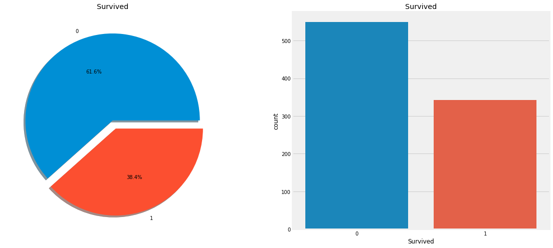
It is evident that not many passengers survived the accident.
Out of 891 passengers in traing set, only around 350 survived i.e Only 38.4% of the total training set survived the crash. We need to dig down more to get better insights from the data and see which categories of the passengers did survive and who didn’t.
We will try to chek the survival rate by using the different features of the dataset. Some of the features being Sex, Port Of Embarcation, Age, etc.
First let us understand the different types of features.
*** Types Of Features**
Categorical Features: A categorical variable is one that has two or more categories and each value in that feature can be categorised by them. For example, gender is a categorical variable having two categories(male and female). Now we cannot sort or give any ordering to such variables. They are also known as Nominal Variables(명목형 변수).
Categorical Features in the dataset: Sex, Embarked
Ordinal Features: An ordinal variable is similar to categorical values, but the difference between them is that we can have relative ordering or sorting between the values. For eg: if we have a feature like Height with values Tall, Medium, Short, then Height is a ordinal variable. Here we can have a relative sort in the variable.
Ordinal(순위) Features in the dataset: PClass
Continuous Feature: A feature is said to be continous if it can take values between any two points or between the minimun or maximum values in the features column.
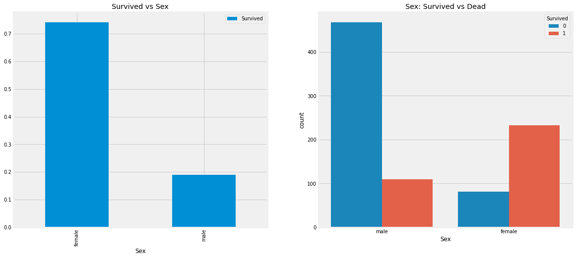
This looks interesting. The number of men on the ship is lot more than the number of women. Still the number of women saved is almost twice the number of males saved. The survival rates for a women on the ship is around 75% while that for men in around 18-19%.
This looks to be a very important feature for modeling. But is it the best? Let’s check other features.
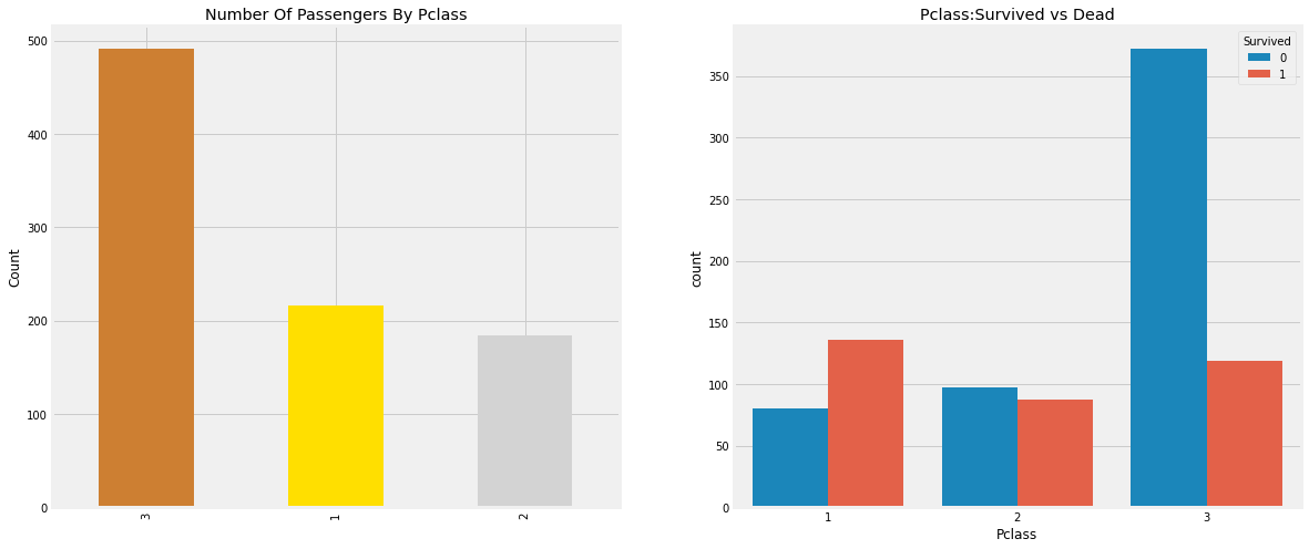
*** Pclass -> Ordinal Feature**
1 2
# 클래스별 사망자/생존자 수 pd.crosstab(train.Pclass, train.Survived, margins=True).style.background_gradient(cmap = 'summer_r')
People say Money Can’t Buy Everything. But we can clearly see that Passengers Of Pclass 1 were given a very high priority while rescue. Even thouugh the number of Passengers in Pclass 3 were a lot higher, still the number of survival from them is very low, somewhere around 25%.
For Pclass 1% survived is around 63% while for Pclass 2 is around 48%. So money and status matters. Such a materialistic world.
Let’s dive in little bit more and check for other interesting observations. Let’s check survival rate with Sex and Pclass Together.
1 2
# Sex, Pclss 기준으로 Survived 인원 보기 pd.crosstab([train.Sex, train.Survived], train.Pclass, margins=True).style.background_gradient(cmap='summer_r')
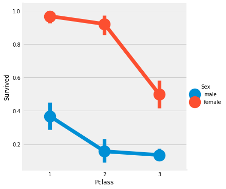
sns.factorplot('Pclass', 'Survived', hue = 'Sex', data = train) plt.show()
We use FactorPlot in this case, because they make the seperation of categorical values easy.
Looking at the CrossTab and the FactorPlot, we can easily infer that survival for Women from Pclass 1 is about 95-96%, as only 3 out of 94 Women from Pclass 1 died.
It is evident that irrespective of Pclass, Women were given first priority while rescue. Even Men from Pclass 1 have a very low survival rate.
Looks like Pclass is also an important feature. Let’s analyse other features.
*** Age -> Continous Feature**
1 2 3
print('Oldest Passenger was of:', train['Age'].max(), 'Years') print('Youngest Passenger was of:', train['Age'].min(), 'Years') print('Average Age on the ship:', train['Age'].mean(), 'Years')
Oldest Passenger was of: 80.0 Years
Youngest Passenger was of: 0.42 Years
Average Age on the ship: 29.69911764705882 Years
1 2 3 4 5 6 7 8
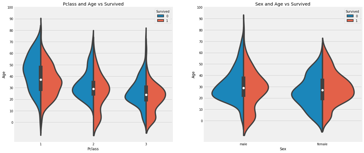
f, ax = plt.subplots(1, 2, figsize = (18, 8)) sns.violinplot("Pclass", "Age", hue="Survived", data=train, split=True, ax=ax[0]) ax[0].set_title('Pclass and Age vs Survived') ax[0].set_yticks(range(0, 110, 10)) sns.violinplot("Sex", "Age", hue="Survived", data=train, split=True, ax=ax[1]) ax[1].set_title('Sex and Age vs Survived') ax[1].set_yticks(range(0, 110, 10)) plt.show()
Observations:
The number of cildren increases with Pclass and the survival rate for passengers below Age 10(i.e children) looks to be good irrespective of the Pclass.
Survival chances for passengers aged 20-50 from Pclass 1 is high and is even better for women.
For males, the survival chances decreases with an increase in age.
As we had seen earlier, the Age feature has 177 null values. To replace these NaN values, we can assign them the mean age of the dataset.
But the problem is, there were many people with many different ages. We just can’t assign a 4 year kid with the mean age that is 29 years. Is there any way to find out what age-band does the passenger lie?
We can check the Name feature. Looking upon the feature, we cas see that the names have a salutaion like Mr or Mrs. Thus we can assign the mean values of Mr and Mrs to the respective groups.
“What’s in a name?” —-> Feature
1 2 3
train['Initial']=0 for i in train: train['Initial']=train.Name.str.extract('([A-Za-z]+)\.') # extract the Salutations
Using the Regex: [A-Za-z]+).. So what it does is, it looks for strings which lie between A-Z or a-z and followed by a .(dot). So we successfully extract the Initials from the Name.
1
pd.crosstab(train.Initial, train.Sex).T.style.background_gradient(cmap='summer_r') # checking the Initials with the sex
train.groupby('Initial')['Age'].mean() # check the average age by Initials
Initial
Master 4.574167
Miss 21.860000
Mr 32.739609
Mrs 35.981818
Other 45.888889
Name: Age, dtype: float64
Filling NaN Ages
1 2 3 4 5 6
# assigning the NaN Values with the Ceil values of the mean ages train.loc[(train.Age.isnull())&(train.Initial=='Mr'),'Age']=33 train.loc[(train.Age.isnull())&(train.Initial=='Mrs'),'Age']=36 train.loc[(train.Age.isnull())&(train.Initial=='Master'),'Age']=5 train.loc[(train.Age.isnull())&(train.Initial=='Miss'),'Age']=22 train.loc[(train.Age.isnull())&(train.Initial=='Other'),'Age']=46
1
train.Age.isnull().any() # so no null values left finally
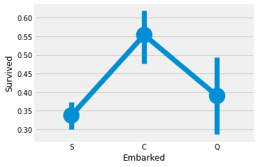
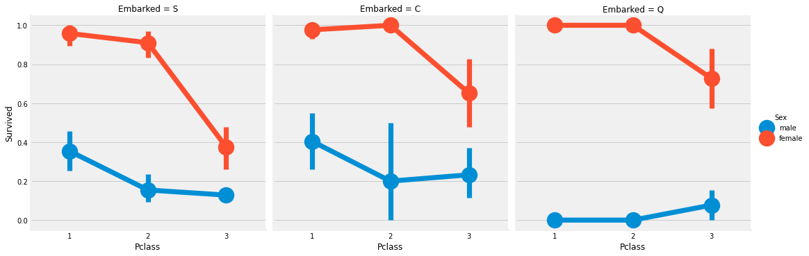
The chances for survival for Port C is highest around 0.55 while it is lowest for S.
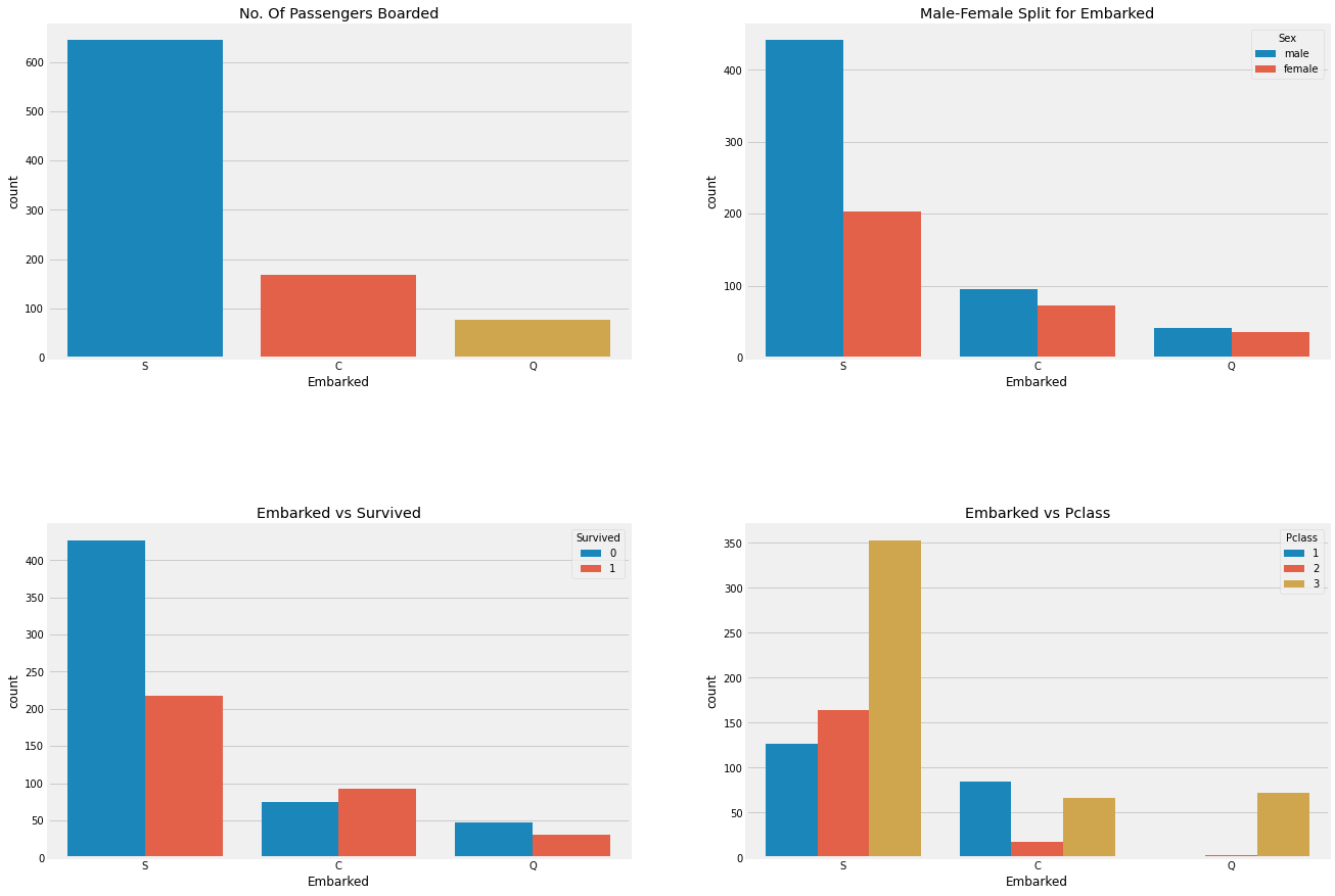
1 2 3 4 5 6 7 8 9 10 11
f,ax=plt.subplots(2,2,figsize=(20,15))
sns.countplot('Embarked',data=train,ax=ax[0,0])
ax[0,0].set_title('No. Of Passengers Boarded')
sns.countplot('Embarked',hue='Sex',data=train,ax=ax[0,1])
ax[0,1].set_title('Male-Female Split for Embarked')
sns.countplot('Embarked',hue='Survived',data=train,ax=ax[1,0])
ax[1,0].set_title('Embarked vs Survived')
sns.countplot('Embarked',hue='Pclass',data=train,ax=ax[1,1])
ax[1,1].set_title('Embarked vs Pclass')
plt.subplots_adjust(wspace=0.2,hspace=0.5)
plt.show()
Observations:
Maximum passengers boarded from S. Majority of them being from Pclass3.
The passengers from C look to be lucky as a good proportion of them survived. The reason for this maybe the rescue of all the Pclass 1 and Pclass 2 passengers.
The Embark S looks to the port from where majority of the rich people boarded. Still the chances for surical is low here, that is vecause many passengers from Pclass 3 around 81% didn’t survive.
Port Q had almost 95% of the passengers were from Pclass 3.