Since I started Kaggle competitions, I have a question. I called it beginner’s curiosity.
“Have you ever thought about which countries have the biggest impact on Kaggle competition?”
As everybody knows, USA is an obvious IT powerhouse along with Silicon Valley. It has the largest number of Kaggle Grandmaster Champions. There is no doubt that the USA has the most influence on Kaggle competitions.
You can also see a lot of Indians on the list of participants. India, known as the rising IT powerhouse, is interested in the Kaggle competitions. It can be confirmed easily by checking a percentage of respondents to the 《2020 Kaggle Machine Learning & data Science Survey》. The response rate for Indians is the highest about 29.2%(5,850 people). It is higher than the second-ranked country, which I would explain.
In addition, a few years ago, every country emphasized the importance of machine learning because It can be used in lots of fields in the world. I also wondered about the future of machine learning, so I decided to look into the future of Machine Learning through responses from two leader countries. Actually, if we look at the current trend of machine learning, we can easily discover it.
“Do you know the future of Machine Learning?”
To sum up, I will compare the responses of American and Indian especially about Machine Learning in the order below.
/opt/conda/lib/python3.7/site-packages/IPython/core/interactiveshell.py:3063: DtypeWarning: Columns (0) have mixed types.Specify dtype option on import or set low_memory=False.
  interactivity=interactivity, compiler=compiler, result=result)
1
2
3
4
5
6
7
8
# Extract data by country
India = df[df['Q3']=='India']
India = India.iloc[1:,:]
India.reset_index(drop=True, inplace=True)

USA = df[df['Q3']=='USA']
USA = USA.iloc[1:,:]
USA.reset_index(drop=True, inplace=True)
1
question.head()
Time from Start to Finish (seconds)                                Duration (in seconds)
Q1                                                           What is your age (# years)?
Q2                                                What is your gender? - Selected Choice
Q3                                             In which country do you currently reside?
Q4                                     What is the highest level of formal education ...
Name: 0, dtype: object
The response rate for Indians is the highest which is about 29.2% or 5,850 people. It is about 2.6 times higher than USA, a second-ranked country. Based on the response of the Americans and Indians for this report, I extracted the data by 2 using the two countries.
Preprocessing
To organize the data neatly, I pre-processed a gender column in which only females and males would remain. (146 responses will be deleted)
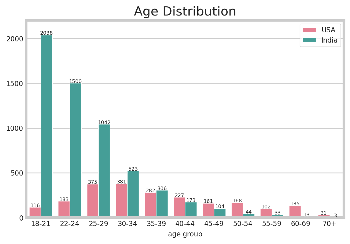
You can easily notice in USA the distribution of age groups is more regular than India. It represents the cording fever especially among young Indians. It can be interpreted that India has a craze for coding.
# male percentage for i in df_q2q3_ratio.index: ax.annotate(f"{df_q2q3_ratio['Man'][i]*100:.3}%", xy=(df_q2q3_ratio['Man'][i]/2, i), fontsize=12, va='center')
for i in df_q2q3_ratio.index: ax.annotate(f"{df_q2q3_ratio['Woman'][i]*100:.3}%", xy=(df_q2q3_ratio['Man'][i]+df_q2q3_ratio['Woman'][i]/2, i), va='center', ha='center', fontsize=12) plt.title('Gender Distribution', fontsize=20)
for s in ['top', 'left', 'right', 'bottom']: ax.spines[s].set_visible(False) ax.legend(loc='lower center', ncol=2, bbox_to_anchor=(0.5, -0.40)) plt.show()
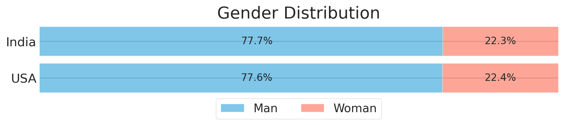
The gender ratio of two countries is alike. In both countries, male respondents are about 3.4 times more than female respondents.
3. Education & Job
Then I checked their education level and their current job.
3-1. Level of Education
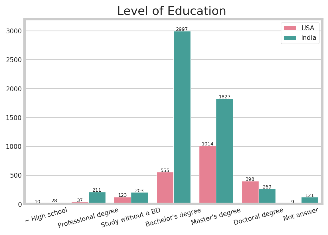
Please notice that I can just confirm their degree level, not major. However, many respondents study above bachelor’s degree, so I think it is okay to assume that their major is related to coding or programming.
df['Q4'] = df['Q4'].str.replace("[^A-Za-z0-9-\s]+", "") df['Q4'].replace({'No formal education past high school':'~ High school', 'I prefer not to answer':'Not answer', 'Some collegeuniversity study without earning a bachelors degree':'Study without a BD', 'Masters degree':"Master's degree", 'Bachelors degree':"Bachelor's degree", ' High school':'~ High school'}, inplace=True)
defcountplot_(data, col_name, q_order): values = data[col_name].value_counts()[q_order].values ax = sns.countplot(x = col_name, hue=data.columns[3], data=data, hue_order = legend_list, palette = "husl", order = ['~ High school', 'Professional degree', 'Study without a BD', "Bachelor's degree","Master's degree",'Doctoral degree', 'Not answer']) for p in ax.patches: height = p.get_height() ax.text(p.get_x() + p.get_width()/2., height+3, height, ha='center', size=6) ax.set_ylim([0, 3200]) plt.xticks(rotation=15, fontsize=8) plt.xlabel('') plt.yticks(fontsize=8) plt.ylabel('') plt.legend(fontsize=8, loc='upper right') plt.title('Level of Education ', fontsize=15) plt.show() q4_order = ['~ High school', 'Professional degree', 'Study without a BD', "Bachelor's degree","Master's degree",'Doctoral degree', 'Not answer'] col_name = "Q4" countplot_(df, col_name, q4_order)
In the case of master and doctor, the percentage of Americans(46.9%, 18.4%) is higher than Indians (31.6%, 4.7%). Many Indians obtained their bachelor’s degree(51.9%) and I also noticed that 3.7% of the Indians had a professional degree.
It shows that USA already has many IT technicians that are highly educated, and India’s level of coding education is growing.
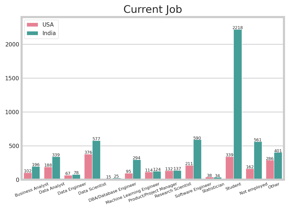
Most noticeably, more than 38% of Indians are students. That’s because 61.2% of the respondents in India are under 25. In the USA, there are lots of Data Scientists(17.4%), and Software Engineers(9.8%). Likewise, India has a lot of Sotfware Engineers(10.2%), and Data Scientists(10.0%). The results of the fewest jobs are the same, too. Both of the countries have few DBA/Database Engineers and Statisticians.
4. Development Environment
In this part, I examined a more detailed part of the development environment. Compared to the period of coding, I discovered each country’s interest in writing code or programming. Furthermore, I will check their basic programming languages and the languages recommended by people who already used it.
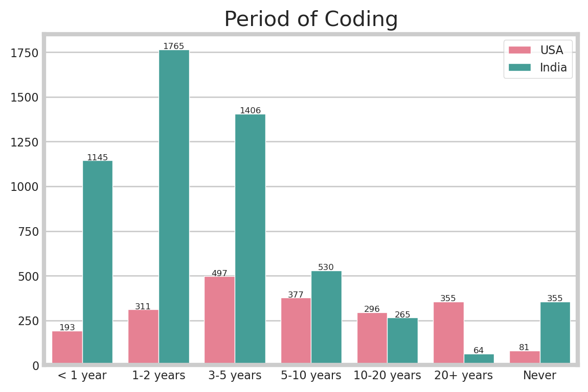
In the case of the USA respondents, the number of people who have never coded nor programmed is less than that of other groups. It show us that Americans have always been interested in it. More than 30.1% of the respondents are experts who have coded for more than 10 years. Additionally, it is noticeable that the number of beginners is decreasing.
India, on the other hand, has about 6.1% of respondents who have never done coding nor programming. Plus, there are numerous beginners. Almost 74.6% of Indians studied coding for less than 5 years, and about half of the respondents in India coded for less than 3 years.
This graph also shows that there are already lots of coding masters in the USA, and that there are many beginners in India.
4-2. Basic programming language (multiple)
1 2 3 4 5 6 7 8 9 10
# Preprocess Basic programming language data USA7 = (USA['Q7_Part_1'], USA['Q7_Part_2'], USA['Q7_Part_3'], USA['Q7_Part_4'], USA['Q7_Part_5'], USA['Q7_Part_6'], USA['Q7_Part_7'], USA['Q7_Part_8'], USA['Q7_OTHER']) USA7 = pd.concat(USA7)
USA7.value_counts().plot.pie(autopct='%.1f%%', ax = ax[0]) ax[0].set_title('Basic Program Language in USA', fontsize=20) ax[0].set_ylabel('')
India7.value_counts().plot.pie(autopct='%.1f%%', ax = ax[1]) ax[1].set_title('Basic Program Language in India', fontsize=20) ax[1].set_ylabel('')
plt.tight_layout() plt.show()
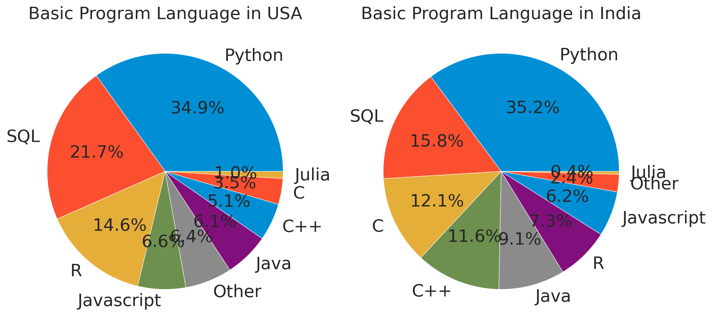
Both countries use Python the most. The next is SQL. A noticeable difference is shown in the 3rd most used language. In the USA, 14.6% of respondents use R, but in India the 3rd most used programming language is C. In India, R is the third- lowest programming language used whereas in the USA, C is the second-lowest.
Nevertheless, it is clear that the most commonly used languages of both countries are Python and SQL.
f, ax = plt.subplots(1, 2, figsize = (12, 8)) USA9.value_counts().plot.pie(autopct='%.1f%%', ax = ax[0]) ax[0].set_title('Using IDE in USA', fontsize=20) ax[0].set_ylabel('')
India9.value_counts().plot.pie(autopct='%.1f%%', ax = ax[1]) ax[1].set_title('Using IDE in India', fontsize=20) ax[1].set_ylabel('')
plt.tight_layout() plt.show()
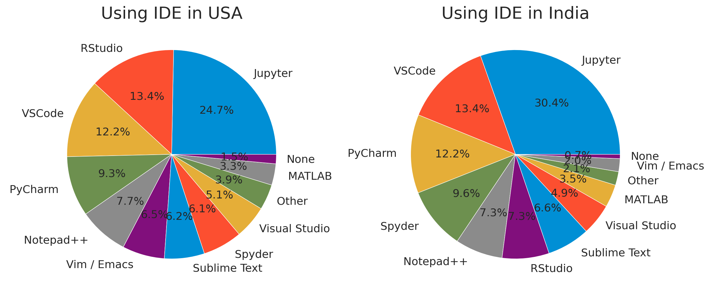
The development environment used frequently is similar except for RStudio. As we saw in 4-2, the reason why the ratio of RStudio in India is not high is Indian less use R.
5. Basic of Machine Learning
It’s time to check the machine learning section. First, I check to period of using machine learning in each country. And then, let’s look at the machine learning framework and algorithms that they use.
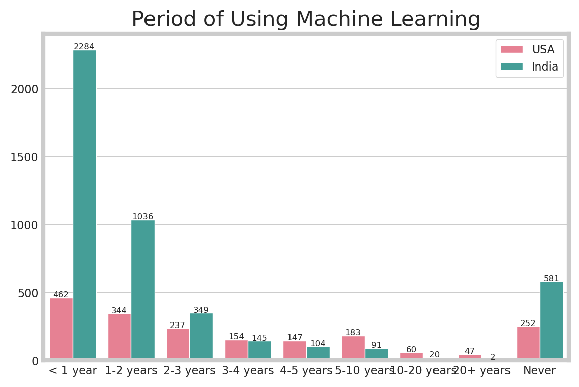
The results of this graph shows the two countries similar. In the USA, many people have been coding for a long time, but there are many beginners in machine learning. Expecially in India, there are about 57.4% of respondents using machine learning. It can be said that India’s coding craze began with the development of machine learning.
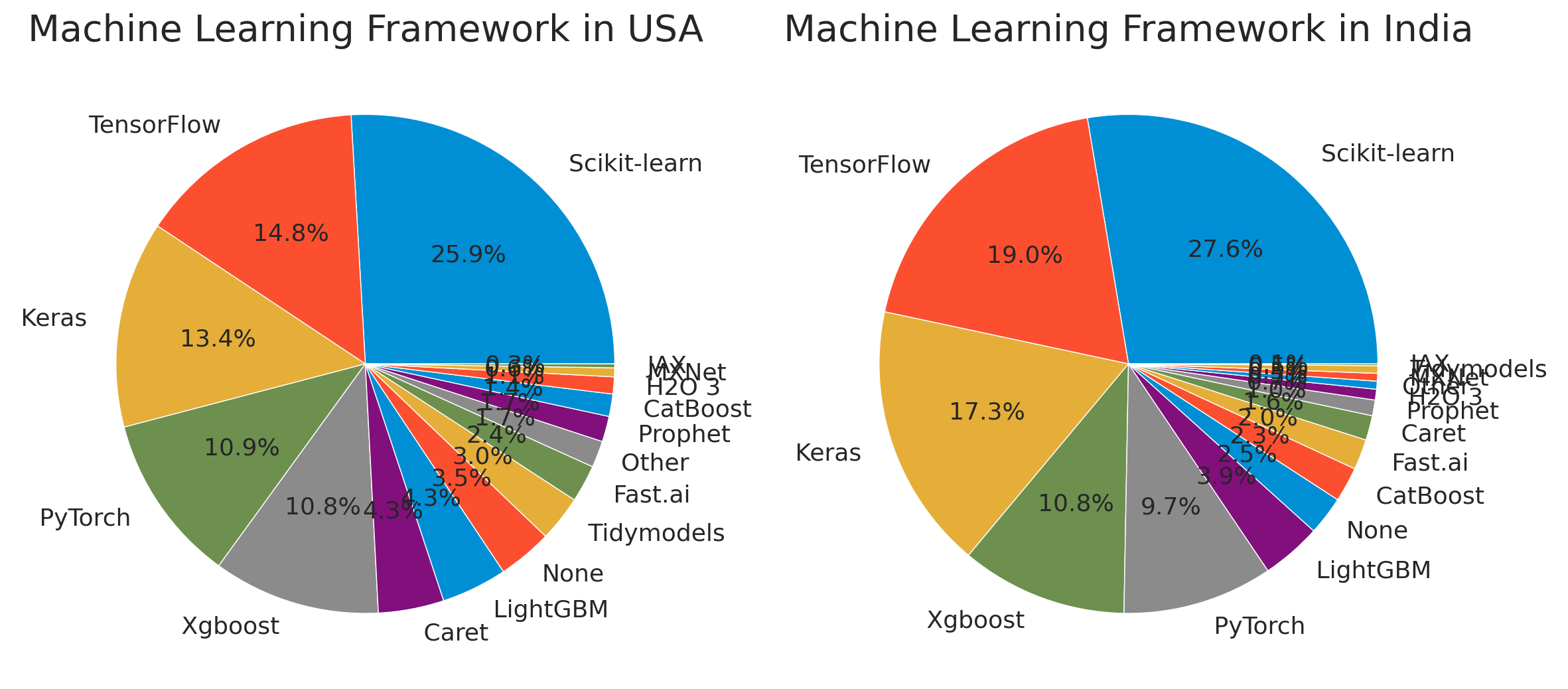
The ranking of machine learning framework of both countries is almost similar. There is a difference between the rank 4th and 5th graphs which is PyTorch and Xgboost. The most popular framework used is Scikit-learn, with about 25.9% in the USA and about 27.6% in India. TensorFlow and Keras showed about 14.5%, and about 13.4% in the USA and in India about 19.0% and about 17.3% are observed. It shows that more than three quarters of people uses 5 types of framework and one quarter of people uses various framework which occupy less than about 10% each.
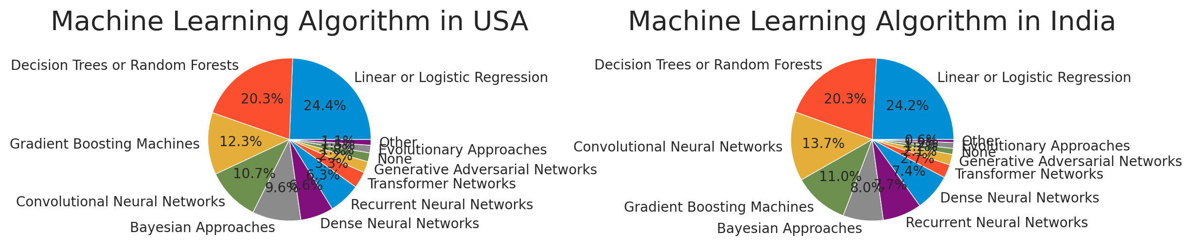
The ranking of used machine learning algorithm of both countries is almost similar, too. Linear or logistic regression and decision trees or random forests are most popular in two countries. And there are no significant thing because the result of both countries is alike.
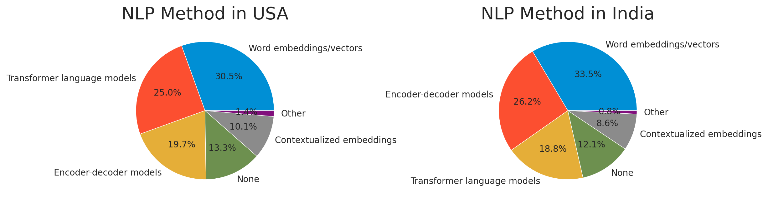
6. CV & NLP
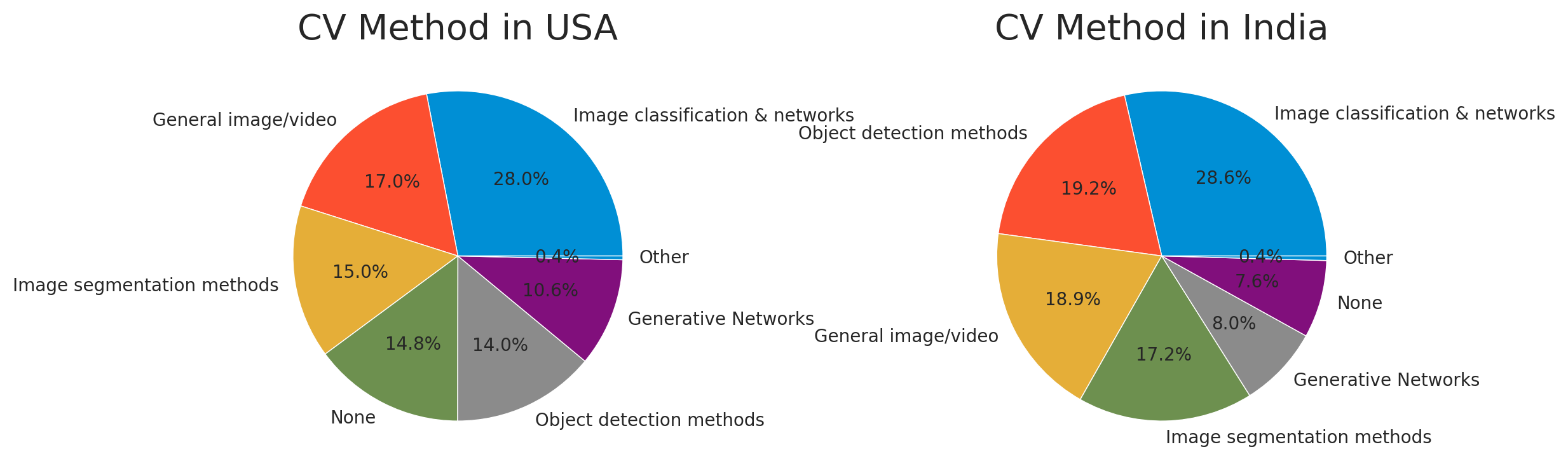
Then, I check about Computer Vision and Natural Language Processing because it is importance part of machine learning. Therefore I assumed lots of beginners and exports are interested in this field. In this part, the difference between the USA and India is not visible clearly, so I just show you the ratio graphs.
USA19.value_counts().plot.pie(autopct='%.1f%%', ax = ax[0]) ax[0].set_title('NLP Method in USA', fontsize=20) ax[0].set_ylabel('')
India19.value_counts().plot.pie(autopct='%.1f%%', ax = ax[1]) ax[1].set_title('NLP Method in India', fontsize=20) ax[1].set_ylabel('')
plt.tight_layout() plt.show()
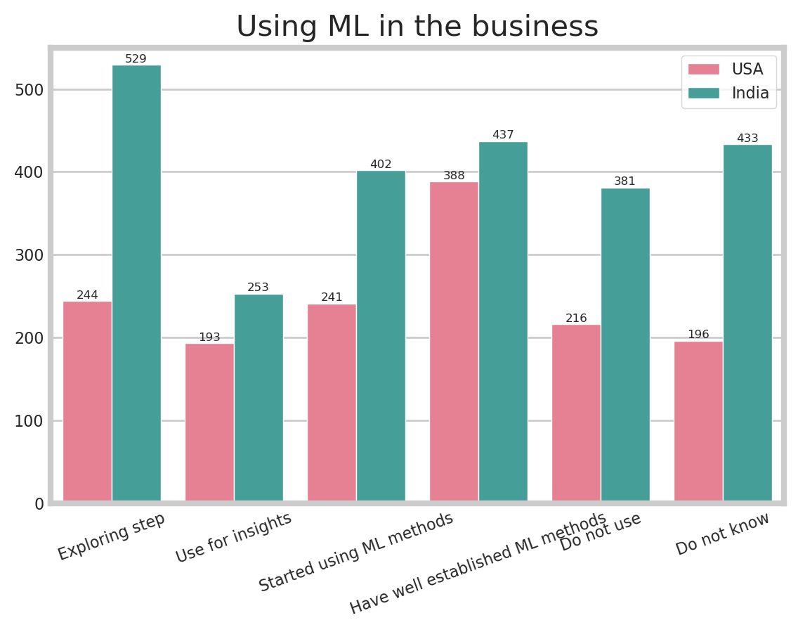
7. Machine Learning in the business
I wondered if the company actually uses machine learning in their business, so I choose this question. Unfortunately, there are few answers that could be used because there are many missing values.
df['Q22'].replace({'We are exploring ML methods (and may one day put a model into production)':'Exploring step', 'We use ML methods for generating insights (but do not put working models into production)':'Use for insights', 'We recently started using ML methods (i.e., models in production for less than 2 years)':'Started using ML methods', 'We have well established ML methods (i.e., models in production for more than 2 years)':'Have well established ML methods', 'No (we do not use ML methods)':'Do not use', 'I do not know':'Do not know'}, inplace=True)
defcountplot_(data, col_name, q_order): values = data[col_name].value_counts()[q_order].values ax = sns.countplot(x = col_name, hue=data.columns[3], data=data, hue_order = legend_list, palette = "husl", order = ['Exploring step','Use for insights','Started using ML methods','Have well established ML methods','Do not use','Do not know']) for p in ax.patches: height = p.get_height() ax.text(p.get_x() + p.get_width()/2., height+3, height, ha='center', size=6) ax.set_ylim([0, 550]) plt.xticks(rotation=20, fontsize=8) plt.xlabel('') plt.yticks(fontsize=8) plt.ylabel('') plt.legend(fontsize=8, loc='upper right') plt.title('Using ML in the business', fontsize=15) plt.show() q22_order = ['Exploring step','Use for insights','Started using ML methods','Have well established ML methods','Do not use','Do not know'] col_name = "Q22" countplot_(df, col_name, q22_order)
There are so many NaN. I think they didn’t know about it, so they just skipped that question. I dropped all NaN in this question.
In the USA, there are about 72.3% of respondents’s firm use machine learning for their business. In India there are about 66.4% of respondents’s firm use it for their business. It is noticeable that the ratio of using machine learning in the business in both counrty is not big different.
However, it may be an uncertain value because all missing values are deleted. Therefore if you wondered about it, I strongly recommend find some useful reports.
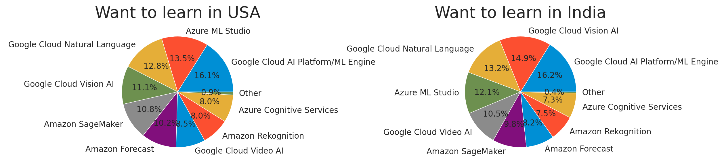
8. Want to learn machine learning product (multiple)
Finally, I comfirm that the machine learning products what Americans and Indians want to learn. Because the importance and potential of machine learning is continuosly emphasized, I feel like it help us to understand the trend of indusrty.
USA28b.replace({' Azure Machine Learning Studio ':'Azure ML Studio', ' Google Cloud AI Platform / Google Cloud ML Engine':'Google Cloud AI Platform/ML Engine'}, inplace=True) India28b.replace({' Azure Machine Learning Studio ':'Azure ML Studio', ' Google Cloud AI Platform / Google Cloud ML Engine':'Google Cloud AI Platform/ML Engine'}, inplace=True) USA28b.value_counts().plot.pie(autopct='%.1f%%', ax = ax[0]) ax[0].set_title('Want to learn in USA', fontsize=20) ax[0].set_ylabel('')
India28b.value_counts().plot.pie(autopct='%.1f%%', ax = ax[1]) ax[1].set_title('Want to learn in India', fontsize=20) ax[1].set_ylabel('')
plt.tight_layout() plt.show()
Everything was chosen by similarly ratio. Above all, Google Cloud AI Platform / Google Cloud ML Engine is the most popular among beginners in two countries.
Conclusion
Through exploratory data analysis of 《2020 Kaggle Machine Learning & df Science Survey》, we were able to learn about trends of coding and machine learning. Comparing with an obvious IT powerhouse country, the USA and the rising IT powerhouse India is very meaningful to explore trends of it. Most noticeable is that the USA has been interested in coding and programs from long ago, and India is a country with coding craze especially among young ages. It is amazing that the two countries’ response are very similar in the part of machine learning surveys. I think it is proven the importance of machine learning these days. It was an interesting work.